Optimizing anamorphic sculptures

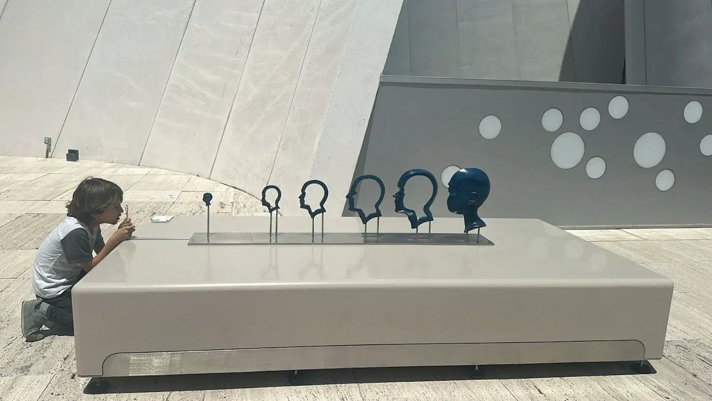
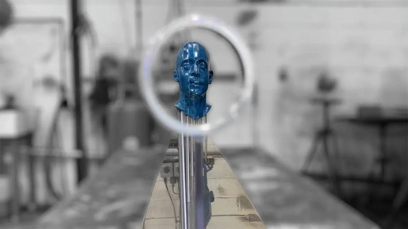
Dozens of car, pig and pigeon meshes floating in space, lining up into the outline of a pig from a single viewpoint. — A pig made of cars, pigs and pigeons.

At my workplace there’s an anamorphic sculpture that reveals a recognizable image only when viewed from a specific vantage point. The work of Jonty Hurwitz explores that technique with mirrors (catoptric anamorphosis) and with perspective (oblique anamorphosis). In Blue Singularity, Jonty’s own head sculpture is displayed in slices. Those slices compose the head when looking from a specific angle.

A child looking at an anamorphic sculpture from the vantage point. It shows different slices of a head that completes the image only from the vantage point. — Blue Singularity from Jonty Hurwitz

The resulting blue sculpture head when seeing from the vantage point. — The sculpture as seen by the vantage point. Blue Singularity from Jonty Hurwitz

My office’s sculpture always gets me thinking about how I would optimize for that kind of result. To experiment with that, I wrote an application that, given a set of 3d meshes, arrange them in the 3d space so that a target silhouette is rendered from a specific camera angle.

A pig made of cars, pigs and pigeons.

Random meshes in, a silhouette out

Sculptures are generated by optimizing the position, size, and rotation of different meshes with gradient descent. Meshes are placed randomly in the scene, the scene silhouette is rendered. The render is then compared to a target image, a loss is computed, and errors are backpropagated to the input parameters (meshes positions, rotations, and scale). At each step meshes are moved and adjusted so the rendered silhouette comes closer to the target image.

Overview of the optimization process. Meshes are placed at random, the silhouette is rendered and compared to the target image.

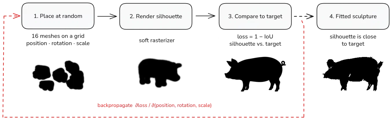
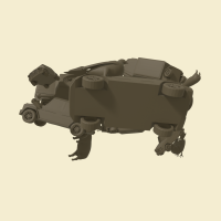
Although the process has few steps, the implementation is not simple. There are multiple implementation details necessary to generate visually interesting images. First and most important, to be able to backpropagate errors from the loss to the input, the rendering step should be differentiable. The loss function should also be tuned to value details. In other words, just getting most of the image right is not enough to get a similar silhouette.

The rasterizer has no gradients

A rasterizer is a function that maps vertices to pixels. It is responsible for converting a list of triangles (3d mesh) into an image. For every pixel it asks whether that pixel is covered by the triangle. This is a binary operation: covered or not. Nudging a triangle slightly changes nothing until its edge crosses a pixel center, and then the pixel flips. This means that the derivative is zero almost everywhere and undefined on the boundary. To backpropagate errors in this setting, some constraints need to be relaxed. Luckily, Liu et al. had this problem before and published a paper on soft rasterizers.

The main idea in SoftRas is to replace the boolean (pixel inside or outside triangle) with a sigmoid of the signed squared distance to the triangle’s boundary. For pixel $i$ and triangle $j$, let $d_{ij}$ be the distance from the pixel center to the triangle’s outline, $\delta_{ij}$ = +1 if inside, -1 if outside triangle, and $\sigma$ a constant to control the transition. Then the “belonging” of a pixel in a triangle can be measured by $p_{ij}$:

$$ p_{ij} = \operatorname{sigmoid}\!\left(\frac{\delta_{ij}\, d_{ij}^2}{\sigma}\right) $$

Experiment with different $\sigma$ values

Move the pixel center across a triangle edge. A smaller $\sigma$ makes the transition sharper; a larger $\sigma$ lets a missed shape send a gradient farther. A hard rasterizer is the $\sigma$ → 0 limit.

Interactive figure — requires JavaScript.

As you can see, different $\sigma$ values have different trade-offs. With a small $\sigma$, errors are only propagated close to the triangle edge. Meshes placed far away won’t be moved. Having a large $\sigma$ will make the silhouette more diffuse. The adopted solution was to anneal $\sigma$: start large and shrink it as the optimization progresses. A large $\sigma$ is the renderer squinting. The silhouette is a blur, but a mesh far from where it should be still feels a pull. Shrinking $\sigma$ opens the renderer’s eyes and sharpens the edges.

Another optimization was splitting the meshes in bins. Not every pixel should be checked against every triangle. Also recomputing gradients during backprop helps keeping the memory in check.

Edges are what make a silhouette recognizable

The naive approach is to compare the rendered silhouette with the target image and adjust the objects. The problem with that is that although the silhouette can have a lot of “mass” in the center, the edges are what make silhouettes distinguishable. On top of that, I wanted the generated sculptures to be manufacturable in the real world, which meant avoiding collisions between placed components.

The loss function computes a single number that represents how good or bad the current arrangement is. The optimizer’s objective is to make this number smaller by nudging where each object sits, how it is turned, and how big it is. The loss is composed by four different components:

The intersection between the computed silhouette and the target (comparison).
A penalty for painting outside the target silhouette (spill).
The quality of the silhouette edges (outline).
A penalty for colliding objects (collisions).

Comparing silhouettes

To compare silhouettes the Intersection over Union is used. This function is widely used for comparing masks and bounding boxes in different computer vision problems. Given the generated image $\alpha$, and the target image $t$ the IoU is given by:

$$IoU = \dfrac{|\alpha \cap t |}{|\alpha \cup t|}$$

In other words, the pixels shared between the two silhouettes divided by the union of “painted” pixels. To be compatible with loss, $1 - IoU$ is used as the metric. In some experiments, I also added a band IoU loss in which only the surroundings of the silhouette are considered.

Reducing spill

Painting outside of the target silhouette hinders IoU but its impact can be small. Since most of the mass is around the core of the image, small variations in the edges, or around the image, don’t impact the loss sufficiently to generate close enough silhouettes. Adding an additional component to penalize out of place meshes increases the final quality of the image. Given a weight $c$, the total number of pixels in the image $|F|$, the spill is given by the sum of painted pixels outside of the target image:

$$\text{spill} = c \cdot \frac{1}{|F|}\sum_i \alpha_i (1 - t_i)$$

Improving the outline

Even with those components, the generated silhouette can have a jagged edge. For example, the little pigeon feet can leak under the pig silhouette generating spikes in the edge. The outline component adds a penalty for perimeters larger than the target image requires.

To capture that information we use a Total variation (TV) metric. It is the sum, over all pixels, of how sharply the image changes at that pixel.

$$\operatorname{TV}(\alpha) = \sum_{i,j} \sqrt{(\partial_x \alpha)^2 + (\partial_y \alpha)^2 + \epsilon}$$

The outline component of the loss is given by the ratio between the rendered image and the target TV.

$$\text{outline} = \dfrac{TV(\alpha)}{TV(t)}$$

Penalizing collisions

The final component of the loss formula aims to reduce overlap between meshes. This way the sculptures could be really built in the real world with the composition of different objects.

The collision penalty is computed with axis-aligned bounding boxes (AABB) for every pair of objects ($P$ is the set of every pair of objects). With $\text{pen}_{ab}$ being the penetration between objects $a$ and $b$, and $\text{width}_{ab}$ the average frame width in the image.

$$\text{collisions} = \frac{1}{|P|}\sum_{(a,b) \in P} \frac{\text{pen}_{ab}}{\text{width}_{ab}}$$

The implementation optimizes this collision to only compute the metric for pairs that can actually collide, which cuts the cost of each optimization step.

Loss formula

All components are multiplied by a weight and summed together. Given the generated image $\alpha$, and the target image $t$, the hand-tuned weights $c, s, w$ the loss function is given by:

$$ L = \underbrace{\bigl(1 - IoU(\alpha, t)\bigr)}_{comparison} \;+\; c \cdot \underbrace{\frac{1}{|F|}\sum_i \alpha_i (1 - t_i)}_{\text{spill}} \;+\; s \cdot \underbrace{\frac{\operatorname{TV}(\alpha)}{\operatorname{TV}(t)}}_{\text{outline}} \;+\; w \cdot \underbrace{\frac{1}{|P|}\sum_{(a,b) \in P} \frac{\text{pen}_{ab}}{\text{width}_{ab}}}_{\text{collisions}} $$

Optimizing for multiple views

There is an interesting byproduct of this optimization process. It is possible to assemble different images for different camera angles with the same set of objects.

One sculpture with a friendly dog viewpoint and a rabbit assembled from the same components.

In this case, there is an additional restriction. Objects inside the intersection of the two camera frustums are visible from both vantage points, so both target images have to agree on what is painted there. Where they disagree, one of the views ends up with components it never asked for.

To maximize the image freedom, I am using two cameras with a 90 degree angle between them. Cameras’ losses are combined with the harmonic mean, which is pulled down by the worse of the two. The optimizer cannot sharpen the dog by letting the rabbit fall apart.

What I want to render next

Another pig, this time made only of pigeons. From any other angle it is a flock going nowhere.

There are still things to explore: rendering with more components, making the result hold up at angles near the vantage point, and using complementary views better. This is not the first time I used gradient descent for art. I did the same for abstract machine learning art , generating images that fool a classifier while staying recognizable to us. What would you like me to render next?