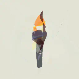
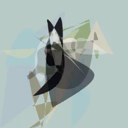
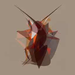
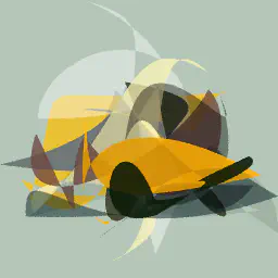
Thiago Cardoso :: Abstract Machine Learning Art

Moving to a new home, I was confronted with empty walls. Thinking about images to decorete them reminded of an old project: creating abstract art using machine learning.

It is fascinating to combine the rigidity of Linear Algebra with art and creativity. Inspired by the work of dribnet , I aimed to create abstract images that could deceive Machine Learning algorithms while still being recognizable to humans. Different from dribnet’s approach, my objective was to generate those images with an end-to-end differentiable approach.

Gif showing the progress of creating an abstract art that represents a cockroach — The evolution of an abstract cockroach.

Given two inputs - a target Imagenet class and a target image - the algorithm optimizes two objectives. The first objective is the difference between the generated image and the target image. The second objective aims to minimize the classification error for the target class, forcing the creation of an image that can be recognized by classification algorithms.

In this example, you can see a piggy bank image. On the right is an image that multiple algorithms correctly classify as piggybank, but it lacks visual grounding for humans. On the left is the image optimized to match the target image.

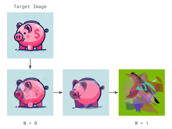
The effect of weight in image optimization. On the left the image that only optimizes for similarity with target, on the right one that is correctly classified as `piggy bank` by multiple models.

Architecture

The main idea is to use diffvg , a differentiable vector graphics rasterizer, for creating the images. This approach allows backpropagation of a given loss to the inputs, adjusting the image to the desired optimization objective. The network input consists of points and colors for each path. Most images in this post are generated with 20 paths. Adding other SVG shapes such as lines, circles or rectangles is planned for future versions.

The diffvg rasterized image is fed into a visual loss and various Machine Learning models to obtain the classification loss. To optimize the image to deceive Machine Learning models, we use different models trained with Imagenet data: AlexNet , VGG11 , and Visual Transformes (ViT_b_16 ), all accessible via Torch Hub. The perceptual similarity (LPIPS ) and RMSE are utilized as the visual losses.

Finally, a loss function weights all the mentioned components. The gradients are backpropagated to the inputs, keeping all models weights frozen. Only the input points and colors are updated. In other words, we are optimizing the generated image to minimize the loss. The following diagram shows the network’s architecture.

flowchart TD
    points[SVG input points]
    colors[SVG input colors]
    target[Target image]
    tcls[Target Imagenet class]
    diffvg[Diffvg]
    image[Rasterized image]
    alexnet[alexnet]
    vgg[vgg11]
    vit[vit_b_16]
    lpips[Perceptual similarity LPIPS]
    rmse[RMSE]
    visual[Visual loss]
    cls[Classification loss]
    loss[Loss function]
    points --> diffvg
    colors --> diffvg
    diffvg --> image
    image --> alexnet
    image --> vgg
    image --> vit
    image --> lpips
    target --> lpips
    target --> rmse
    image --> rmse
    alexnet --> cls
    vgg --> cls
    vit --> cls
    rmse --> visual
    lpips --> visual
    cls --> loss
    tcls --> cls
    visual --> loss

    subgraph Legend
    ni[Network Inputs]
    ui[User Inputs]
    end

    style ni fill:#FFAA80
    style points fill:#FFAA80
    style colors fill:#FFAA80
    style ui fill:#9BEC00
    style target fill:#9BEC00
    style tcls fill:#9BEC00

Loss function

To better understand the optimization process, it’s important to detail the loss function used. This function was refined through experimentation with the objective to create visually interesting art. The loss has two main components: the target class loss and the visual loss. The target class loss measures how far a model is from classifying the image as the target class using cross-entropy . The visual loss measures the distance of the resultant image from the target image. These components are weighted by the hyperparameter $w$. When $w=0$, only the visual loss is considered. When $w=1$, only the target class loss is considered. The complete formula is as follows:

$$ \begin{align} \text{AlexLoss} &= \text{CrossEntropyLoss}_{\text{AlexNet}}(\hat{y}, y) \\ \text{VGGLoss} &= \text{CrossEntropyLoss}_{\text{VGG11}}(\hat{y}, y) \\ \text{VitLoss} &= \text{CrossEntropyLoss}_{\text{Vit_b_16}}(\hat{y}, y) \\ \text{TargetClassLoss} &= \text{mean}(\text{AlexLoss}, \text{VGGLoss}, \text{VitLoss}) \\ &+ \text{sd}(\text{AlexLoss}, \text{VGGLoss}, \text{VitLoss}) \\ \\ \text{VisualLoss} &= \text{LPIPS}(y, \hat{y}) + \text{RMSE}(y, \hat{y}) \\ \\ \text{Loss} &= ((1.0 - w) * \text{VisualLoss}) + (w * \text{TargetClassLoss}) \end{align} $$

The target class component sums the mean with the standard deviation of the losses. Using the standard deviation ensures that all models’ losses are optimized together, preventing significant differences between them. From my tests, this approach yields better results. Removing the standard deviation could cause the optimization to favor one model over another, leading to potential saddle points and stagnation.

To measure the visual difference between images, two loss functions are combined: LPIPS and RMSE between the generated and target images. LPIPS is usually enough for optimizing an image that broadly resembles the target but incorporating RMSE provides better guidance for the optimization process.

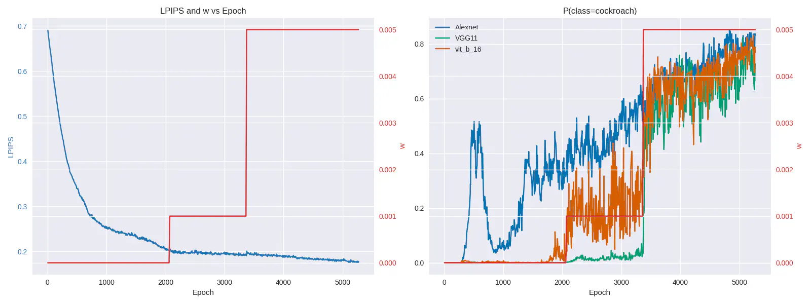
To achieve better results, the weight $w$ should start at zero and increase throughout the process. During the first epochs, the focus should be on optimizing for visual similarity alone. As optimization progresses, the target class component is gradually introduced until the image is predicted as belonging to the target class. No scheduling algorithm is employed; this process is done manually by examining the image and loss charts. The following charts show the progress in LPIPS loss and target classification as well as changes in $w$.

Charts showing the reduction in LPIPS and the increase in target class probability — Progress in LPIPS loss and target classification.

Half art, half engineering

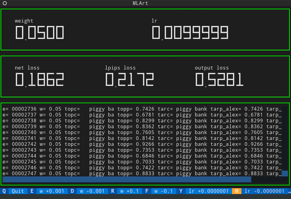
I developed a Terminal User Interface (TUI) that displays logs and important losses, allowing real-time interaction with the algorithm. The TUI provides a comprehensive overview of the optimization process, making it possible to fine-tune the weights interactively without interrupting the optimization workflow. The following screenshot showcases the functionality and layout of the TUI. Losses and metrics are logged using Tensorboard.

Screenshot of TUI that allows for interatction with parameters — TUI for adjusting optimization parameters. It is possible to increment the weight, the learning rate, and read current losses.

Can it fool ChatGPT?

Now you may be asking, do these images actually fool ML models? The models used to generate the images indeed assign high probability to the target class. As more models are incorporated, these adversarial images become more robust. However, the effectiveness varies with other models, depending on their underlying architecture and training data. The following representation of a torch is correctly classified by Alexnet (84%), Vgg11 (79%), and Vit (90%).

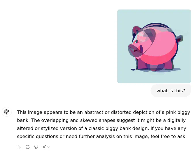
From my examples, I was able to achieve one adversarial example that fools ChatGPT (gpt-4o). In this image, you see a piggy bank image before $w$ was increased. Although it is similar to the final image, ChatGPT couldn’t guess its representation.

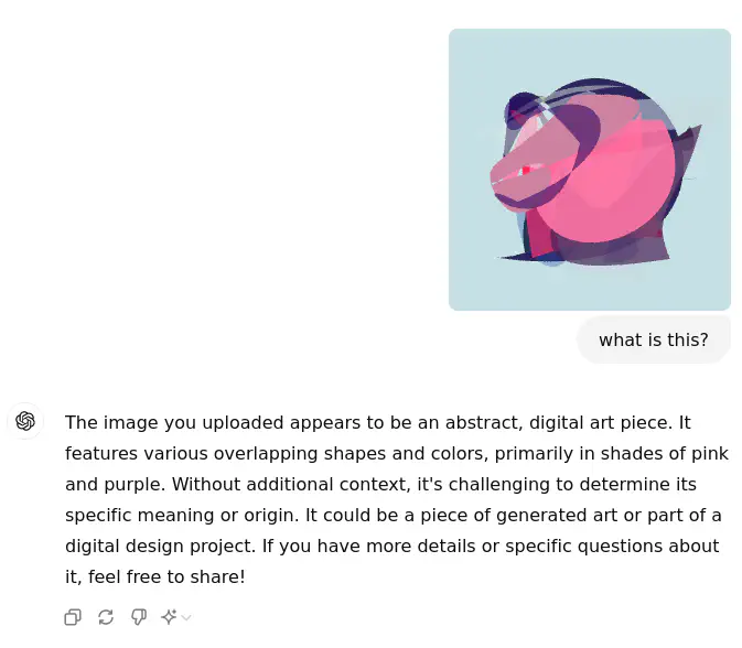
ChatGPT classification of image before increasing w.

After optimizing for the target class, ChatGPT recognizes it as a piggy bank. It is possible to generate adversarial images for ChatGPT, but developing a robust method would require further research.

ChatGPT classification of image after increasing w. ChatGPT is able to see a Piggy Bank.

Gallery